Ising Model

This is a Conformal Field Theory “Hello World” project. Apparently the symmetry group of the ising model around its phase transition is actually the Virasoro group. Therefore we can conformal field theory our way into a nice description about it, just to play around with the fundamental objects there.

We begin with a classical treatment of the model to fully define some terminology (but also because it is fun) and then move on to identify how the matching with the CFT description occurs.

---

Classical Treatment

Here is a brief overview the classical treatment of the 2D Ising model in order to find the limit at which it reduces to a quantum model.

Physical Setting

The setup is a bunch of arrows arranged in a lattice that can interact with their nearest neighbors. A picture is the following, where we have a 2D lattice and an arrow attached at each point.

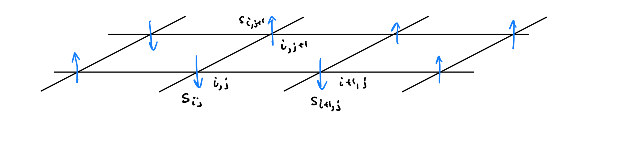
To build a mathematical description of the model, we can first identify a suitable configuration space. Let’s start with a finite lattice 2D lattice that contains a total of $N=n^2$ particles. This can be described as ${\mathbb{Z}}_n^2$, where at each point of which we have attached a spin up or down vector in ${\mathbb{Z}}_2$ for the vector space. Therefore the configuration space is given by

$$C_N:={\mathbb{Z}}_n^2\times {\mathbb{Z}}_2.$$

Notice that ${\mathbb{Z}}_n^2$ as a graph admits the topology of a discrete donut! That is because we can connect the endpoints of the grid for each ${\mathbb{Z}}_n$. The next ingredient we need is a Hamiltonian $H:C_N\to \mathbb{R}$.

The Hamiltonian in this case must capture the interaction of the neighboring spins. For some point $p=(s_1,s_2,\cdots ,s_N)\in C_N$ we usually pick the Hamiltonian

$$H(p)=-\sum _{i,j}{J}_{ij}{s}_i{s}_j-h\sum _i{s}_i$$

where $J$ is an $N\times N$ symmetric matrix such that $J_{ij}=I>0$ iff $s_i$ is neighboring $s_j$, otherwise $J_{ij}=0$, and $h>0$ represents some external magnetic field type interaction. Note that $s_i\in \{-1,1\}$. Now we are ready to calculate the magnetization in the Canonical ensemble.

Magnetization in the Canonical Ensemble

In the Canonical Ensemble, the partition function is given by

$$Z=\sum _{p\in C_N}{e}^{-\beta H(p)}$$

Classically the magnetization is given by the average of the particles aligned in the up direction like so

$$M=\frac{1}{N\beta }⟨s_T⟩=\frac{1}{N\beta }\sum _{i=0}^N⟨s_i⟩=\frac{1}{N\beta }\frac{\partial }{\partial h}\log Z.$$

The phase transition also appears on the susceptibility which is given by

$$\chi ={\frac{\partial M}{\partial h}|}_{h=0}=\frac{1}{N\beta }{\frac{{\partial }^2}{\partial h^2}|}_{h=0}\log Z$$

With some algebraic manipulation we can get that

$$\chi =\frac{1}{N\beta }[-\frac{1}{Z^2}{\left(\frac{\partial Z}{\partial h}\right)}^2+\frac{1}{Z}\frac{{\partial }^{2}Z}{\partial h^2}]=\frac{\beta }{N}[⟨s_{{\rm T}}^2⟩-⟨s_{{\rm T}}{⟩}^2]=\frac{\beta }{N}\text{Var}(s_{{\rm T}})$$

OK! All of this is not quantum, but check out that

$$\text{Var}\left[\sum _{i=0}^N{s}_i\right]=\sum _{i,j=0}^n\text{Cov}(s_i,s_j)=\sum _{i,j=0}^n⟨s_i{s}_j⟩-⟨s_i⟩⟨s_j⟩$$

The cool thing is that $s_i,s_j$ are uncorrelated unless $i,j$ are neighbors. Therefore we can write this a sum of the uncorrelated differences, which depends only on $|i-j|$ which hints to translation invariance, and a really cool use of CFT!

We will use CFT to calculate these correlation functions.

Mean Field Theory During Transition

---

Quantum Treatment

Ok, everything up to now has been fun, but it has mostly been background so that when we treat Ising in CFT we can be like OH COOL! Look at these conformal weights! They are the same as the classical ones! Now we will proceed with establishing a correspondence between the classical Ising model and some CFT. We do this by establishing a connection between the classical treatment and the quantum treatment and then we take a continuum limit of the quantum model to some CFT. So before we do everything there let's understand the Quantum Ising model.

Classical Starting Point

This whole section can be skipped if you don't care about rigorously motivating angular momentum in classical Hamiltonian mechanics.

Let's first consider the single spin case in 3D. We have a magnetic moment $\mu$ with fixed magnitude and the only thing we care about is its direction. This is the picture of the classical situation.

The only quantity of interest is this angular momentum vector $\mu$, which transforms under a representation of $SO(3)$. In practice, in our physics we don't care about anything other than the orientation of this magnetic moment. Therefore, we can safely say that the configuration space is just a sphere! We could show this nicely by performing a symplectic reduction of $T^{\ast }{\mathbb{R}}^3$.

For the purposes of this construction we will consider the spin as a point in $S^2$, with the symplectic form $\omega$ given by its embedding in $i:S^2\to {\mathbb{R}}^3$ like so

$$\omega =i^{\ast }{\iota }_{n}d\text{vol},$$

where $d\text{vol}$ is the standard volume form of ${\mathbb{R}}^3$ and $n\in \mathfrak{X}({\mathbb{R}}^3)$ is any vector field that is perpendicular to the surface of the sphere. This induces a nondegenerate symplectic form that is the volume form on the sphere given by

$$\omega =\sin \theta d\theta \wedge d\varphi ,$$

where $\theta ,\varphi$ are the standard coordinates on the sphere.

The first thing that we want to show is to find the momentum map of the sphere.

Proposition: The restriction on the sphere of the fundamental representation of $SO(3)$ on ${\mathbb{R}}^3$ is a Hamiltonian action on $S^2$ with momentum map the inclusion map $\iota :S^2\to {\mathbb{R}}^3\cong \mathfrak{so}(3)$.

Proof: We will show that $X_x,X_y,X_z$ follow the standard commutation relations of the generators of $SO(3)$.

In particular we want to show that

$$\begin{array}{r}\{q^i,q^j\}={ϵ}_k^{ij}{q}^k.\end{array}$$

We can now calculate that

$$\begin{array}{rl}\{q^i,q^j\}& ={\iota }_{X_{q^j}}{\iota }_{X_{q^i}}\omega \\ & ={\iota }_{X_{q^j}}{\iota }_{X_{q^i}}{i}^{\ast }{\iota }_{n}d\text{vol}\end{array}$$ $$\begin{array}{}◻& \end{array}$$

In fact here is a picture of their Hamiltonian vector fields for $x,y,$ and $z$ respectively.

Now we can move on through geometric quantization to produce the Hilbert space associated to this thing.

Hamiltonian

Now consider the Hamiltonian of that spin system. If the point on the sphere is an angular momentum, then on an external magnetic field $H\in {\mathbb{R}}^3$ the Hamiltonian is given by $H:S^2\to \mathbb{R}$

$$H(p)=q^i(p)H_i.$$

We can actually plot this Hamiltonian right here,

Where the phase space is shown in translucent gray and the Hamiltonian ($r=H(\varphi ,\theta )$) is shown as the blue sphere. Notice that in this depiction the magnetic field is pointing towards the top. Therefore we can see two unstable extrema parallel to $H$ and two stable ones perpendicular to it.

Interestingly, we can think of what happens when we have $n$ such spins. In that case, the phase space is

$${\mathcal{P}}_n=\{p:{\mathbb{Z}}_n\to S^2\},$$

with the canonical product topology and symplectic form.

We want those to interact with each other, so the way we will do this is using graphs.

Definition: Given a connected graph $G=(V,E)$, the phase space ${\mathcal{P}}_n$ together with the graph is called an interacting system if there exists a bijection $V\to \{{\pi }_i:{\mathcal{P}}_n\to S^2\}$ to the set of canonical projections of ${\mathcal{P}}_n$. If $G$ is a cyclic undirected graph, then the system is called cyclic or nearest neighbor.

Proposition: In a nearest neighbor interacting system there exists a map $J:{\mathcal{P}}_n\to {\mathcal{P}}_n$ such that the set of edges is given by

$$E=\{({\pi }_i,{\pi }_i\circ J)\mid i=1,2,\dots ,n\}.$$

This map is called the adjacency map and it is a permutation.

Now, we can play with the interaction terms. We will restrict our attention to nearest neighbor interacting systems because they have an interesting relation with the quantum mechanical and field theoretic models. In particular, let's say that the spins interact with each other based on their $z$ component. What that means in practice is that the Hamiltonian has a stable extremum when the spins are aligned in the $z$ direction. We will formalize it like so:

Proposition: Given a map $f:S^2\to V$, where $V$ is some vector space, the map lifts to a unique map $\overline{f}:{\mathcal{P}}_n\to V^n$ such that the following diagram commutes.

$$\begin{array}{ccc}{\mathcal{P}}_n& \stackrel{\overline{f}}{\to }& V^n\\ {\iota }_i\uparrow & & \downarrow {\pi }_i& \\ S^2& \stackrel{f}{\to }& V\end{array}$$

Proof: The map is $\overline{f}=\underset{n\text{ times}}{\underbrace{f\times f\times \cdots \times f}}$.

$$\begin{array}{}◻& \end{array}$$

Proposition: The map $f$ lifts to a map $J_f:{\mathcal{P}}_n\to V^n$ such that

$$J_f(p)=\sum _{(i,j)\in E}{\iota }_j\circ f\circ {\pi }_i(p).$$

In the case the system is nearest neighbor, we have that $J_f$ is given by $J_f=f^{\ast }J=\overline{f}\circ J$.

In other words we can introduce the following interaction term:

$$\begin{array}{rl}{H}_I:{\mathcal{P}}_n& \to \mathbb{R}\\ p=(p_1,p_2,\cdots ,p_n)& \mapsto H_I(p):=-J^{ij}z(p_i)z(p_j),\end{array}$$

where $J:{\mathbb{R}}^n\to {\mathbb{R}}^n$ is a symmetric positive definite matrix called the interaction matrix. If $J_{ij}\ne 0$ then we say that $p_i,p_j$ are neighbors. The simplest such interaction matrix would be the following

$$J^{ij}=J({\delta }^{i(j+1)}+{\delta }^{i(j-1)}+{\delta }^{i1}{\delta }^{jn}+{\delta }^{j1}{\delta }^{in}),$$

for some $J>0$. In this scenario we ca write the full Hamiltonian as:

$$\boxed{{\displaystyle H=-H^i{q}_i-J^{ij}{z}_i{z}_j.}}$$

If the external field is pointing in the $x$ direction we have

$$H=-h\sum _{i=0}^n{x}_i-J^{ij}{z}_i{z}_j.$$

Construction of Hilbert Space

Performing canonical quantization we see that $x_i,y_i,z_i$ form representations of $\mathfrak{so}(3)$ respectively. After going through the geometric quantization procedure by polarizing on the $\theta$ coordinate we obtain a 2-dimensional Hilbert space for the single sphere which we can label by the eigenvalues of the representation of the $z$ operator.

Proposition: The single particle Hilbert space ${\mathcal{H}}_1$ is a quantum Hilbert space.

Now we can proceed by defining operators appropriately through geometric quantization by identifying the linear operator $z:{\mathcal{H}}_1\to {\mathcal{H}}_1$. That for the two pure states ${\psi }_{+}=(\genfrac{}{}{0ex}{}{1}{0}),{\psi }_{-}=(\genfrac{}{}{0ex}{}{0}{1})$ it acts as follows

$$\begin{array}{rlrlrlr}z{\psi }_{+}={\psi }_{+}& & z{\psi }_{-}=-{\psi }_{-}& & ⟹& & z={\sigma }_z=\left(\begin{array}{cc}1& 0\\ 0& -1\end{array}\right).\end{array}$$

We can then create the $N$ particle Hilbert space by taking tensor products like so:

previousDefinition: The $N$ particle Hilbert space is given by ${\mathcal{H}}_N:=\underset{n=1}{\overset{N}{⨂}}{\mathcal{H}}_1$. And the $i$th spin operator $z_i:{\mathcal{H}}_N\to {\mathcal{H}}_N$ is given by

$$z_i=1\otimes 1\otimes \cdots \underset{i^{\text{th}}\text{ position}}{\underbrace{\otimes z\otimes }}\cdots \otimes 1.$$

So now we have the Hilbert space constructed and we can proceed with the Hamiltonian.

Definition: The Quantum $N$ particle Ising Hamiltonian is the linear map $H:{\mathcal{H}}_N\to {\mathcal{H}}_N$ given by

$$H=H_1+H_0=-J^{ij}{z}_i{z}_j-h\sum _{i=0}^N{x}_i$$

where $x_i={\sigma }_{xi}$ is the corresponding operator to the $x_i:{\mathcal{P}}_n\to \mathbb{R}$ map, with the commutation relations that we are expecting. Notice that $[H_1,H_0]\ne 0$.

Quantum to Classical Correspondence

The item of interest that will facilitate the correspondence of the the classical and the quantum theories is the partition function. We have calculated it for the 2-dimensional Ising model in the previous section, so we can try to evaluate it for this one.

The partition function is given by

$$Z=\mathrm{Tr}{e}^{-\beta H}.$$

for some $\beta \ge 0$. However we see that to do this we need to somehow calculate

$$e^{-\beta (H_0+H_1)},$$

which are non-commuting operators. We could use Baker-Campbell-Hausdorff to obtain the result, but that is insane. Anyway here is the proposition.

Proposition: The partition function is given by

$$Z={\mathrm{\Lambda }}^{NL}\sum _{z_i,z_j=\pm 1}{e}^{\mathrm{\Delta }\tau J^{ij}{z}_i{z}_j+\gamma \sum _{i,j}^{N,L}{z}_j{z}_j}$$

for some $L\in \mathbb{N}$, and $\mathrm{\Lambda },\gamma \in \mathbb{R}$.

Quantum Field Theory

Having the quantum mechanical model it is time to "take the continuum limit" and obtain a quantum field theory for it. This is done through the Jordan-Wigner transformation that we will explore in mode detail. What we will derive, is a prescription to increase the number of spins in such a way that it limits to the CFT of a free fermion.

To do so, we will define linear operators $c_i:\mathcal{H}\to \mathcal{H}$ such that

$$\begin{array}{rlr}{\sigma }_i^z=-\prod _{i<j}(1-2c_j^{†}{c}_j)(c_i+c_i^{†})& & {\sigma }_i^x=1-2c_i^{†}{c}_i.\end{array}$$

Proposition: These operators have the following commutation relations

1. $\{c_i,c_j^{†}\}={\delta }_{ij}$
2. $\{c_i,c_j\}=\{c_i^{†},c_j^{†}\}=0$

The cool thing is that we can now rewrite the Hamiltonian.

Proposition: The Hamiltonian for the 1D Ising chain can be written as

$$H=-J\sum _{i=1}^N{c}_i^{†}{c}_{i+1}+c_{i+1}^{†}{c}_i+c_i^{†}{c}_{i+1}^{†}+c_{i+1}{c}_i-2gc{i}^{†}{c}_i+g.$$

Proof: Plug it in and cry.

$$\begin{array}{}◻& \end{array}$$